The Problem in Symbols

The way that we express this is in terms of true positives and true negatives. A true positive is a case where we classify someone as having mastery and that person actually had mastery. A true negative is a case where we classify someone as not having mastery and that person actually does not have mastery. And keep in mind that our rules for classification are observing whether or not the person got the majority of questions correct.

In symbols we have the following:

\[\text{Accuracy} = \frac{\left|\text{True Positives}\right| + \left|\text{True Negatives}\right|}{\left|\text{All Observations} \right|}\]

The formula says that accuracy is the sum of the numbers of all the true positives and true negatives divided by the number of all observations in total. The vertical bars (i.e. \(\left|\ldots\right|\)) represent the size of the object inside, in this case the size of those sets so named.

Now how often does each of these happen? Some notation:

1. \(P(x)\) denotes the probability of x.
2. \(P(x \vert y)\) denotes the probability of x given y.
3. Abbreviations:
   • TP: True Positive
   • TN: True Negative
   • M: Mastery
   • NM: Nonmastery
   • CAM: Classify as Mastery
   • CANM: Classify as Nonmastery.

OK, now we can break down the problem. First, we have \(\left|\text{TP}\right| = \left|\text{All Observations}\right|P(M)P(C\!A\!M\vert M)\). This is because the product \(\left|\text{All Observations}\right|P(M)\) is the number of positive (i.e. mastery) observations and \(P(C\!A\!M\vert M)\) is the fraction of positive (i.e. mastery) observations which are classified as mastery.

Similarly, we have \(\left|\text{TN}\right| = \left|\text{All Observations}\right|P(N\!M)P(C\!A\!N\!M \vert N\!M)\). Because a nonmastery observation must either be classified as mastery or nonmastery and because all observations must either be from people possessing mastery or nonmastery, we have \(P(M) + P(N\!M) = 1\) and \(P(C\!A\!M\vert N\!M) + P(C\!A\!N\!M \vert NM) = 1\). Combined with the problems’ stating that there are equal numbers of people with mastery and nonmastery, we have \(P(M) = P(N\!M) = \frac{1}{2}\).

Substituting these deductions back into our formula for accuracy, we have the following:

\[\text{Accuracy} = \frac{\left|\text{All Observations}\right|P(M)P(C\!A\!M\vert M) + \left|\text{All Observations}\right|P(N\!M)P(C\!A\!N\!M \vert N\!M)}{\left|\text{All Observations} \right|}\]

\[\text{Accuracy} = P(M)P(C\!A\!M\vert M) + P(N\!M)P(C\!A\!N\!M \vert N\!M)\]

\[\text{Accuracy} = \frac{1}{2}P(C\!A\!M\vert M) + \frac{1}{2}(1 - P(C\!A\!M\vert N\!M))\]

\[\text{Accuracy} = \frac{1}{2}(1 + P(C\!A\!M\vert M) - P(C\!A\!M\vert N\!M))\]

And this formula hopefully makes sense. According to intuition, as the number of questions on the exam increases \(P(C\!A\!M\vert M)\) approaches 1 and \(P(C\!A\!M\vert N\!M)\) approaches 0, so our accuracy approaches 1.

Simulating The Rate of Classifying as Mastery Given Nonmastery

Understand that both of these unknown terms can be functions of other parameters, such as how many questions we choose to include on the exam. In fact, fixing the number of questions on the exam will allow us to give actual values in place of these terms.

We can express the equational form of accuracy in R code as follows:

accuracy <- function(p_cam_given_mastery, p_cam_given_nonmastery) {
  (1/2)*(1 + p_cam_given_mastery - p_cam_given_nonmastery)
}

What exactly is \(P(C\!A\!M\vert N\!M)\)? Again, that is the rate at which someone who is guessing gets a majority of questions correct. We can use the R function rbinom in order to simulate exams.

rbinom(n = 10, size = 8, prob = 1/4)

##  [1] 3 1 2 2 3 0 4 4 3 3

Here we have simulated 10 exams each with 8 questions, each individual question having a 1/4 chance of being answered correctly. The 10 numbers shown represent the number of correct responses in each exam. So we can do this for a large number of simulations and observe the result:

library(ggplot2)

## Registered S3 methods overwritten by 'ggplot2':
##   method         from 
##   [.quosures     rlang
##   c.quosures     rlang
##   print.quosures rlang

sims <- data.frame(num_questions = 1:30)
p_cam_given_nm <- function(q_count) sum(rbinom(n = 1e6, size = q_count, prob = 1/4) > (q_count/2))/(1e6)
sims$cam_given_nm_rate <- unlist(Map(p_cam_given_nm, sims$num_questions))
ggplot(data = sims, mapping = aes(x = num_questions, y = cam_given_nm_rate)) +
  geom_line() +
  geom_point() +
  ggtitle("Rate of Classification as Mastery Given Nonmastery") +
  ylab("Rate") +
  xlab("Number of Questions on the Exam") +
  theme_classic()

Great, so now we can see the rates that we classify as having mastery given nonmastery for the various exam lengths. A quick couple of sanity checks:

1. On an exam with one question, we classify as mastery 1/4 of the time. This makes sense because a person with nonmastery answers a single question correctly 1/4 of the time.
2. On an exam with two questions, we classify as mastery 1/16 of the time. This makes sense because a person with nonmastery answers both questions in the two-question-exam correctly 1/16 = (1/4)*(1/4) of the time.

Simulating The Rate of Classifying as Mastery Given Mastery

Now what about \(P(C\!A\!M\vert M)\)? Again we can use rbinom to simulate exams. But in this case, we have some uncertainty about what the probability of a person having mastery answering a question correctly is. Call this probability a person’s aptitude. An aptitude could be anything in the interval greater than 50% and less than or equal to 100%. We can certainly simulate exams by sampling aptitudes first, but crucially, we have to make an assumption about the distribution of aptitudes.

We will go through four scenarios. Aptitudes will be sampled…

1. uniformly from 50% to 100%,
2. clustered more heavily around 50%,
3. clustered more heavily around 100%,
4. normally and centered on 75%.

In this case, we need a function that will help us truncate those probabilities which lie outside of the acceptable 50% to 100% range. Then we will calculate and visually verify the distributions of aptitudes in the four scenarios:

truncate_prob <- function(p) {
  too_low <- which(p < .5)
  too_high <- which(p > 1)
  if (length(too_low) > 0) {
    p[too_low] <- .5
  }
  if (length(too_high) > 0) {
    p[too_high] <- 1
  }
  return(p)
}
aptitudes_scenario_1 <- runif(n = 1e4, min = .5, max = 1)
aptitudes_scenario_2 <- truncate_prob(.5 + rexp(1e4)/20)
aptitudes_scenario_3 <- truncate_prob(1 - rexp(1e4)/20)
aptitudes_scenario_4 <- truncate_prob(rnorm(n = 1e4, mean = .75, sd = .1))
hist(aptitudes_scenario_1, breaks = 60)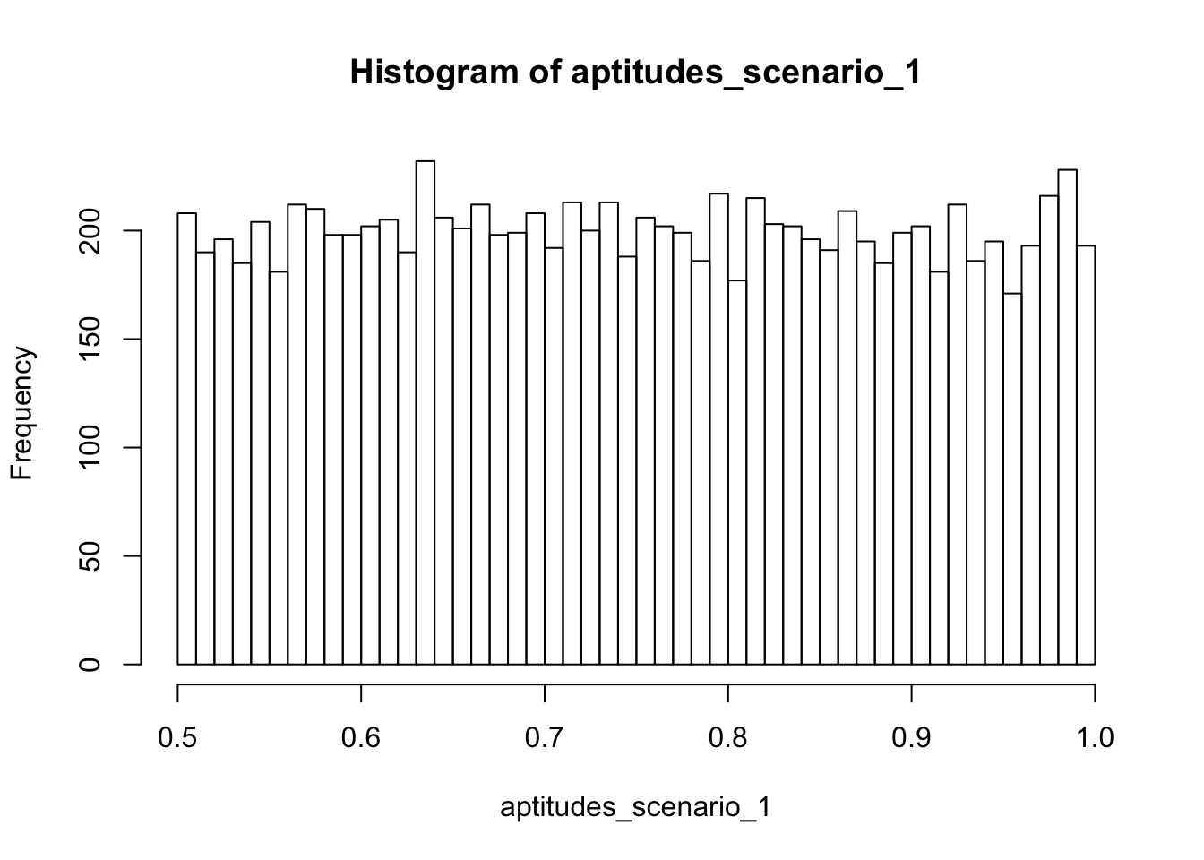

hist(aptitudes_scenario_2, breaks = 60)

hist(aptitudes_scenario_3, breaks = 60)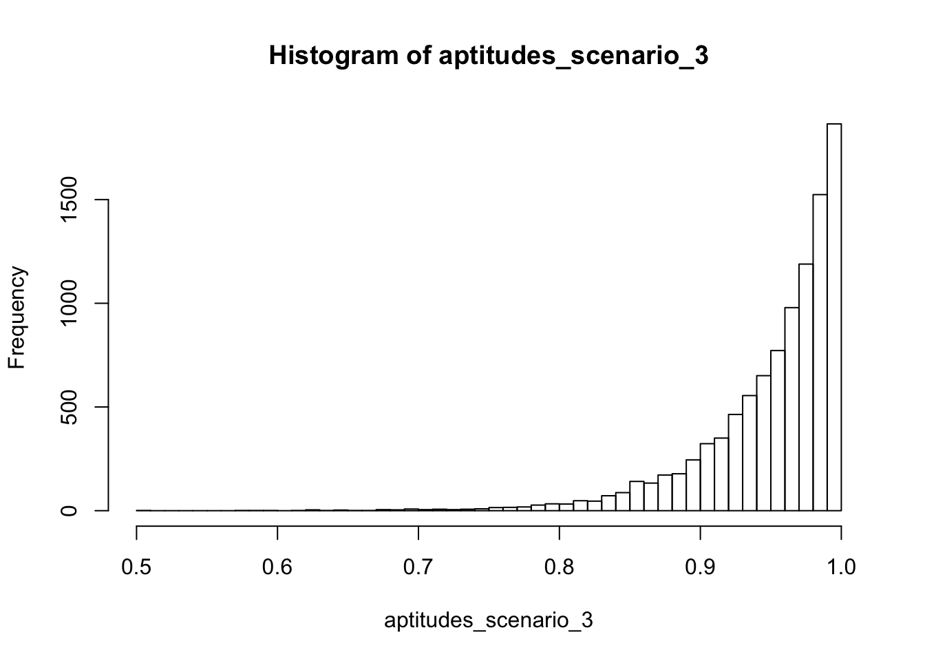

hist(aptitudes_scenario_4, breaks = 60)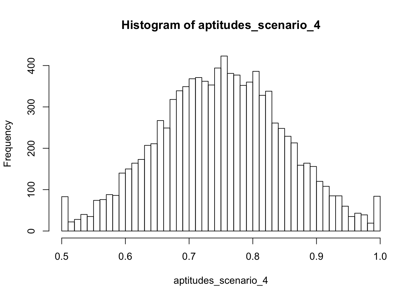

To me, each scenario looks like the text description of what it was supposed to resemble. Scenario 1 contains aptitudes that are evenly spread around the entire range. Scenario 2 clusters at the low end and slowly drops off. Scenario 3 clusters at the high end and drops off as aptitudes decrease. And scenario 4 has many aptitudes around the midpoint of the range, dropping off as we move away in either direction.

Notably, scenario 4 contains spikes at 50% and 100% corresponding with our truncation. These spikes could correspond to some post facto heuristic justification such as the prevalence of over-studiers (high end spike) or perhaps those students who got extra credit after the fact (low end spike). Coming up with these post facto justifications is often a challenging but fun part of the job of telling a story with data. When doing exploratory data analysis on fresh data sets, we are often challenged with interpreting patterns such as these spikes which defy our prior expectations.

The function to sample exams takes the same form as before. In this case, I increased the number of exam simulations from one million to ten million because we are increasing some uncertainty over the aptitudes as well. Also I am defining some helper functions for each different scenario of aptitude sampling. The helper functions are just for brevity and readability of code.

p_cam_given_m <- function(q_count, p) {
  sum(rbinom(n = 1e7, size = q_count, prob = p) > (q_count/2))/(1e7)
}
p_cam_given_m_s1 <- function(q_count) p_cam_given_m(q_count, p = aptitudes_scenario_1)
p_cam_given_m_s2 <- function(q_count) p_cam_given_m(q_count, p = aptitudes_scenario_2)
p_cam_given_m_s3 <- function(q_count) p_cam_given_m(q_count, p = aptitudes_scenario_3)
p_cam_given_m_s4 <- function(q_count) p_cam_given_m(q_count, p = aptitudes_scenario_4)
sims$cam_given_m_s1_rate <- Map(p_cam_given_m_s1, q_count = sims$num_questions)
sims$cam_given_m_s2_rate <- Map(p_cam_given_m_s2, q_count = sims$num_questions)
sims$cam_given_m_s3_rate <- Map(p_cam_given_m_s3, q_count = sims$num_questions)
sims$cam_given_m_s4_rate <- Map(p_cam_given_m_s4, q_count = sims$num_questions)

Now to visualize the classification as mastery rates for those students with mastery:

library(tidyr)
sims_long <- gather(sims, scenario, cam_rate, -num_questions)
sims_long$cam_rate <- unlist(sims_long$cam_rate)
sims_long$label <- ""
sims_long$label[sims_long$scenario == "cam_given_nm_rate"] <- "Nonmastery"
sims_long$label[sims_long$scenario == "cam_given_m_s1_rate"] <- "Mastery -- S. 1"
sims_long$label[sims_long$scenario == "cam_given_m_s2_rate"] <- "Mastery -- S. 2"
sims_long$label[sims_long$scenario == "cam_given_m_s3_rate"] <- "Mastery -- S. 3"
sims_long$label[sims_long$scenario == "cam_given_m_s4_rate"] <- "Mastery -- S. 4"
ggplot(data = sims_long, mapping = aes(x = num_questions, y = cam_rate, color = label)) +
  geom_line() +
  geom_point() +
  ylab("Rate of Classification as Mastery") +
  xlab("Number of Questions on the Exam") +
  guides(color = guide_legend("Aptitude Scenario")) +
  theme_classic()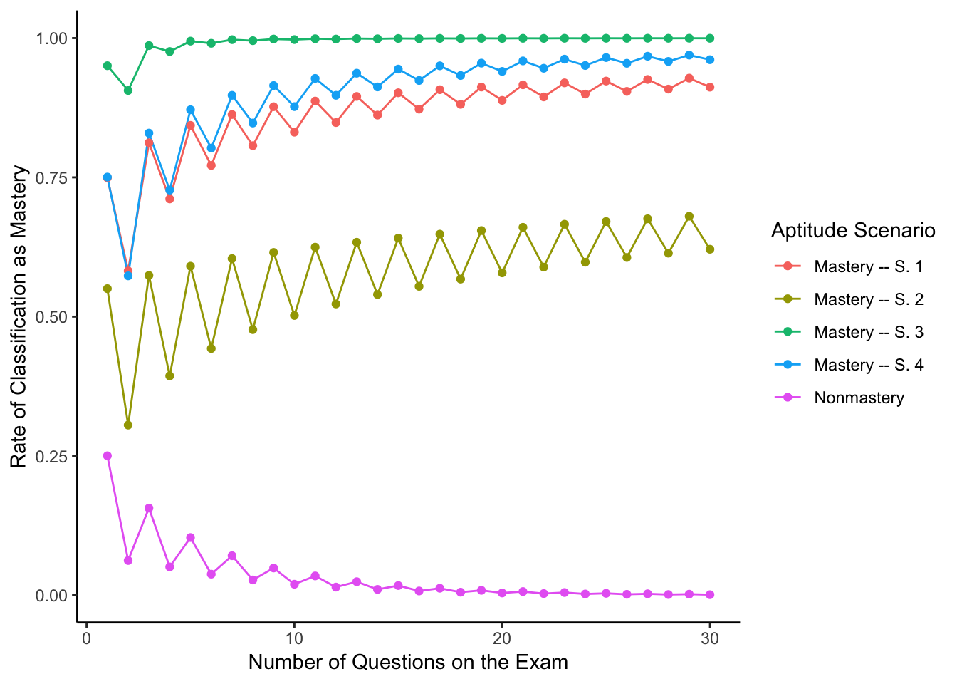

The Moment of Truth

Now that we have estimates of \(P(C\!A\!M\vert M)\) and \(P(C\!A\!M\vert N\!M)\) we can compute accuracies at the different numbers of questions. First, a reminder of our functional form of the accuracy:

accuracy

## function(p_cam_given_mastery, p_cam_given_nonmastery) {
##   (1/2)*(1 + p_cam_given_mastery - p_cam_given_nonmastery)
## }

result <- cbind(sims_long[sims_long$scenario != "cam_given_nm_rate",], cam_rate_given_nonmastery = sims$cam_given_nm_rate)
result$accuracy <- accuracy(result$cam_rate, result$cam_rate_given_nonmastery)
ggplot(data = result, aes(num_questions, accuracy, color = label)) + 
  geom_line() +
  geom_point() +
  geom_hline(yintercept = .95, alpha = .5, linetype = "dashed") +
  #geom_segment(aes(x = 4, xend = 4, y = .5, yend = .96), alpha = .5, linetype = "dashed") +
  scale_x_continuous(expand = c(0,1)) +
  ylab("Rate of Accuracy") +
  xlab("Number of Questions on the Exam") +
  guides(color = guide_legend("Aptitude Scenario")) +
  theme_classic()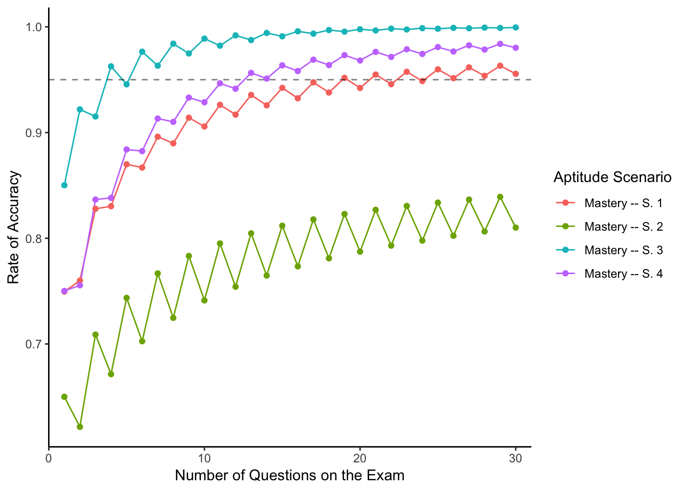

So for our four distributional assumptions of aptitudes of test takers possessing mastery, we have the following results:

1. When aptitudes are evenly spread from 50% to 100%, our exam needs 19 questions.
2. When aptitudes are clustered around 50%, we need many more than 30 questions.
3. When aptitudes are clustered around 100% our exam needs only 4 questions!
4. When aptitudes are normally distributed centered at 75% our exam needs 13 questions.

I think that the scenario where we assume that people with mastery have aptitudes roughly evenly distributed from 50% to 100% is reasonable and conservative. So I would advise the question asker that making her exam 19 questions long would give her a 95% chance of being able to deduce which students possess mastery and which do not.

Question in Review

Some of the topics we reviewed and applied in answering this question:

1. Classification rule
2. Definition of accuracy
3. True positives and true negatives
4. Conditional probability
5. Simulating uncertain scenarios
6. Making decisions under uncertainty
7. Using functional map for iteration instead of imperative for loops
8. Plotting and interpreting results

I hope this post has been interesting or educational for you and you have had fun reading it. Thanks for persevering to the end. If you would like to contact me, feel free to reach out to the links at the top of the web site.