## Registered S3 methods overwritten by 'ggplot2':
##   method         from 
##   [.quosures     rlang
##   c.quosures     rlang
##   print.quosures rlang

Let’s do an integral. What is the total area under the curve $f(x)=x^2$ from $x=-1$ to $x=2$ and from $x=4$ to $x=5$? We typically write this as $\int_{-1}^{2} x^2 \, dx + \int_{4}^{5} x^2 \, dx$. Remembering some elementary calculus, we have $$\int_{-1}^{2} x^2 \, dx + \int_{4}^{5} x^2 \,dx = \\\int_{-1}^{2} \frac{d}{dx} \frac{x^3}{3} \, dx + \int_{4}^{5} \frac{d}{dx} \frac{x^3}{3} = \\\left.\frac{x^3}{3}\right|_{-1}^{2} + \left.\frac{x^3}{3}\right|_{4}^{5} = \frac{70}{3}.$$ So the answer to the question is $\frac{70}{3}$ units of area.

In order to see what’s actually going on here, let’s write a function to plot the curve. Fortunately this is easy as ggplot2 package provides the stat_function function which does most of the work for us.

plot_curve <- function(curve, domain) {
  ggplot() + 
    stat_function(fun = curve, aes(domain, curve(domain))) + 
    geom_vline(xintercept = 0) + 
    geom_hline(yintercept = 0) +
    scale_x_continuous(expand = c(0,0)) +
    ylab("") + xlab("")
}
plot_curve(function(x) x^2, c(-1,5))

So pretty standard stuff. ggplot::stat_function does most of the work here, sampling across the domain of the given function and evaluating for us.

plot_auc <- function(curve, domain, regions) {
  samples <- Map(function(r) data.frame(xs = seq(min(r), max(r), length.out = 100)), regions)
  geoms <- Map(function(s) geom_area(data = s, aes(x = xs, y = curve(xs)), alpha = .5), samples)
  return(Reduce(`%+%`, geoms, init = plot_curve(curve, domain)))
}
plot_auc(curve = function(x) x^2, domain = c(-1,5), regions = list(c(-1,2), c(4,5)))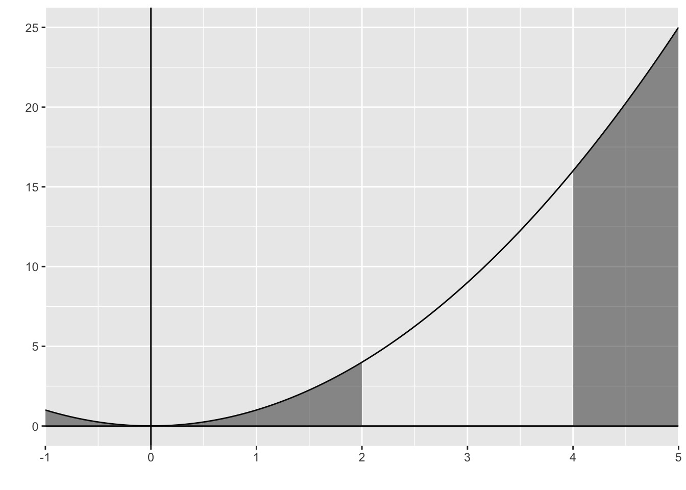

In general it is not easy to find antiderivatives such as above, so we use numerical integration schemes in order to approximate solutions. I will be back in future posts to discuss some methods for doing this.